easyEWAS Tutorial
2025-01-01
easyEWAS.RmdIntroduction
easyEWAS is a user-friendly R package designed for conducting epigenome-wide association studies (EWAS). With easyEWAS, we provide a battery of statistical methods to support differential methylation position analysis across various scenarios, as well as differential methylation region analysis based on the DMRcate method. To facilitate result interpretation, we provide comprehensive functional annotation and result visualization functionalities. Additionally, a bootstrap-based internal validation was incorporated into easyEWAS to ensure the robustness of EWAS results. easyEWAS is compatible with currently most cited Illumina high-density microarray platforms for genome-wide methylation profiling, including 27K, 450K, EPIC V1, EPIC V2, and MSA arrays.

Installation
Users can install the easyEWAS package by running the following code:
devtools::install_github("ytwangZero/easyEWAS")Prepare Data Files
easyEWAS supports only .csv and .xlsx file
formats, so ensure your data is in one of these formats. The package
also includes internal sample and methylation datasets for users to
explore and test its functions.
Sample data: Users need to prepare a sample file to store sample information, such as sample ID, exposure variables, covariates, etc. The sample ID must be the first column, and each ID should be unique and consistent across all files.
data("sampledata", package = "easyEWAS")
head(sampledata)
#>   SampleName var cov1     cov2 batch
#> 1 ZE10000001  76    2 20.96810     1
#> 2 ZE10000002  66    2 26.78373     1
#> 3 ZE10000003  71    2 28.26081     1
#> 4 ZE10000004  81    1 22.54459     1
#> 5 ZE10000005  70    1 21.66550     1
#> 6 ZE10000006  68    2 16.94033     1
Methylation data: Users also need to prepare a methylation file, requiring each row to represent a CpG site and each column to represent a sample. The data format is as follows:
data("methydata", package = "easyEWAS")
head(methydata[,1:6])
#>             probe ZE10000001 ZE10000002 ZE10000003 ZE10000004 ZE10000005
#> 1 cg01444397_BC11 0.04768038 0.02783589 0.02852848 0.06711713 0.04478172
#> 2 cg12110931_TC11 0.43900591 0.43166163 0.51290795 0.45075799 0.59972834
#> 3 cg12258811_TC21 0.41950433 0.47744150 0.52750836 0.53600388 0.64258103
#> 4 cg08764927_TC21 0.82080027 0.82292072 0.88725030 0.87222326 0.91267532
#> 5 cg25514503_TC21 0.94965507 0.95133812 0.95787150 0.96158814 0.96021148
#> 6 cg24454741_TC21 0.88100024 0.89587378 0.90661704 0.88505037 0.86547789
Analysis pipeline
Library the package
library(easyEWAS)Step 1: Initialize the EWAS module
Here, take the easyEWAS internal dataset as an example. After loading
easyEWAS, the user needs to use the initEWAS() function to
initialize an analysis module. This will generate a folder named
EWASresult under the working path specified by the user to
store the EWAS analysis results. If default, the results will be stored
in the current working path. For detailed information on these
parameters, please refer to initEWAS
documentation.
res <- initEWAS(outpath = "default")
#> Complete initializing the EWAS module! Your EWAS results will be stored in D:/R/Rwork/Rpackage/easyEWAS/vignettes/EWASresult
#> 2025-01-03 14:34:07.105257
#> 0.14 sec elapsed
When specifying a custom storage path, make sure that the path actually exists.
res <- initEWAS(outpath = "D:/test")Note: The function returns an R6 object integrating all
information, so the user needs to assign the result of the function to a
new name, such as res.
Step 2: Load the Data Files
Users can upload sample data and methylation data in two ways.
One is to assign the data set in the R environment directly to the
parameters ExpoData and MethyData. If the user
chooses to read data from external sources, the file paths need to be
specified in the parameters ExpoPath and
MethyPath.Detailed information can be found at loadEWAS
documentation.
# Here we read data from the environment.
# Or we can source by specifying file paths:
# ExpoPath = 'D:/DATA/dat1.csv', MethyPath = 'D:/DATA/dat2.csv'
res <- loadEWAS(input = res,
                ExpoData =  sampledata,
                MethyData = methydata)
#> Complete loading All files!
#> 2025-01-03 14:34:07.176157
#> 0 sec elapsed
Note the input parameter, which needs to be
assigned the res generated in the previous step!
Step 3: Transform the variable types
This is an optional step where the user can transform certain variables in the sample dataset to a desired type. The function supports both factor and numeric types. Detailed information can be found at transEWAS documentation.
res <- transEWAS(input = res, Vars = "cov1",TypeTo = "factor")
#> Variable types have been transformed successfully!
#> 0.01 sec elapsed
Step 4: Remove batch effects
This step is optional. Batch effect correction is based on the
ComBat function from the sva package. The sample data provided by the
user must include known batch information. Before correcting for batch
effects, the user can specify the name of the batch in the batch
parameter, as well as the names of the variates of interest and other
covariates besides batch in the adjustVarparameter to avoid
overcorrection. The methylation data stored in
res$Data$Methy will ultimately be replaced with a set of
corrected DNA methylation values, with batch effects effectively
removed. Detailed information can be found at batchEWAS
documentation.
res <- batchEWAS(input = res, adjustVar = "var", batch = "batch")
#> Start to adjust batch effects, please be patient ...
#> Batch effect adjustment has been completed !
#> You can find the adjusted  methylation data in input$Data$Methy.
#> 2025-01-03 14:34:08.907541
#> 1.64 sec elapsed
If plot = TRUE, prior plots will be given with black as
a kernel estimate of the empirical batch effect density and red as the
parametric.
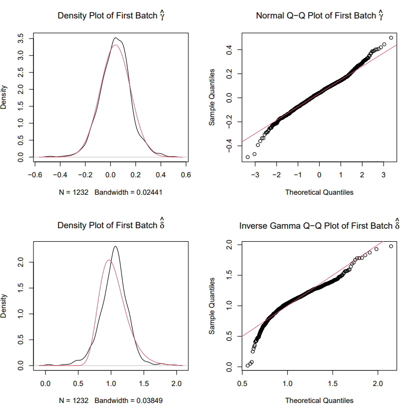
Step 5: Peform the EWAS analysis
This is the core step of the analysis. The user can select
models based on the analysis requirements, including linear regression
models, linear mixed effects models, and Cox proportional risk models.
The results can be exported to a file in working directory. For a
detailed explanation of each parameter, please refer to the package
manual. The startEWAS function supports parallel
operations, and the number of logical cores required for operations can
be specified in the core parameter. Detailed information
can be found at startEWAS
documentation.
parallel::detectCores()-1            # Maximum recommended number of cores
#> [1] 17
res <- startEWAS(input = res,
                chipType = "EPICV2", # "EPICV1", "450K", "27K", "MSA"
                model = "lm",        # "lm", "lmer", "cox"
                expo = "var",        # exposure variable
                cov = "cov1,cov2",   # covariates
                adjustP = TRUE,      # adjust p-values (FDR and Bonferroni)
                random = NULL,       # set only for lmer
                time = NULL,         # set only for Cox
                status = NULL,       # set only for Cox
                core = 10            # set cores for parallel operations
                )
#> It will take some time, please be patient...
#> Start the EWAS analysis...
#> Start multiple testing correction ...
#> Start CpG sites annotation ...
#> EWAS analysis has been completed!
#> You can find results in D:/R/Rwork/Rpackage/easyEWAS/vignettes/EWASresult.
#> 2025-01-03 14:34:34.437661
#> 25.42 sec elapsed
The results can be viewed in res$result.For linear
regression and linear mixed-effects models, when the exposure variable
is continuous, the output includes the coefficient (per unit, per IQR,
per SD), standard error, significance P-value, adjusted P-value, and
annotation for each site. For categorical variables, coefficients are
provided for each class relative to the reference group. In Cox
proportional hazards models, hazard ratios (HR) and confidence intervals
are also included.
head(res$result)
#>             probe          BETA    BETA_perSD   BETA_perIQR           SE
#> 1 cg01444397_BC11  5.724133e-04  5.345447e-03  0.0087293025 1.594601e-04
#> 2 cg12110931_TC11  2.012009e-03  1.878903e-02  0.0306831439 6.058078e-04
#> 3 cg12258811_TC21  1.917825e-04  1.790949e-03  0.0029246826 5.173171e-04
#> 4 cg08764927_TC21 -3.726331e-05 -3.479812e-04 -0.0005682655 4.552721e-04
#> 5 cg25514503_TC21  6.708728e-06  6.264905e-05  0.0001023081 8.123277e-05
#> 6 cg24454741_TC21 -6.095697e-05 -5.692430e-04 -0.0009295938 1.282312e-04
#>       SE_perSD   SE_perIQR         PVAL       FDR Bonfferoni chr     pos
#> 1 0.0014891086 0.002431767 0.0005237102 0.1059711   0.645211   1 7784390
#> 2 0.0056572995 0.009238568 0.0012686133 0.1214434   1.000000   1 7784577
#> 3 0.0048309345 0.007889085 0.7116590121 0.9001683   1.000000   1 7784675
#> 4 0.0042515312 0.006942899 0.9349376448 0.9720196   1.000000   1 7784835
#> 5 0.0007585874 0.001238800 0.9343523148 0.9720196   1.000000   1 7785010
#> 6 0.0011974795 0.001955526 0.6356047918 0.8722169   1.000000   1 7785177
#>   relation_to_island
#> 1             Island
#> 2             Island
#> 3             Island
#> 4             Island
#> 5             Island
#> 6              Shore
#>                                                                    gene
#> 1                          PER3;PER3;PER3;PER3;PER3;PER3;PER3;PER3;PER3
#> 2
#> 3 PER3;PER3;PER3;PER3;PER3;PER3;PER3;PER3;PER3;PER3;PER3;PER3;PER3;PER3
#> 4 PER3;PER3;PER3;PER3;PER3;PER3;PER3;PER3;PER3;PER3;PER3;PER3;PER3;PER3
#> 5
#> 6
#>                                                                              location
#> 1                              5UTR;exon_1;5UTR;exon_1;5UTR;exon_1;5UTR;exon_1;TSS200
#> 2
#> 3 5UTR;exon_2;5UTR;exon_2;5UTR;exon_2;5UTR;exon_2;5UTR;exon_2;5UTR;exon_2;5UTR;exon_2
#> 4 5UTR;exon_2;5UTR;exon_2;5UTR;exon_2;5UTR;exon_2;5UTR;exon_2;5UTR;exon_2;5UTR;exon_2
#> 5
#> 6
Downstream Analysis
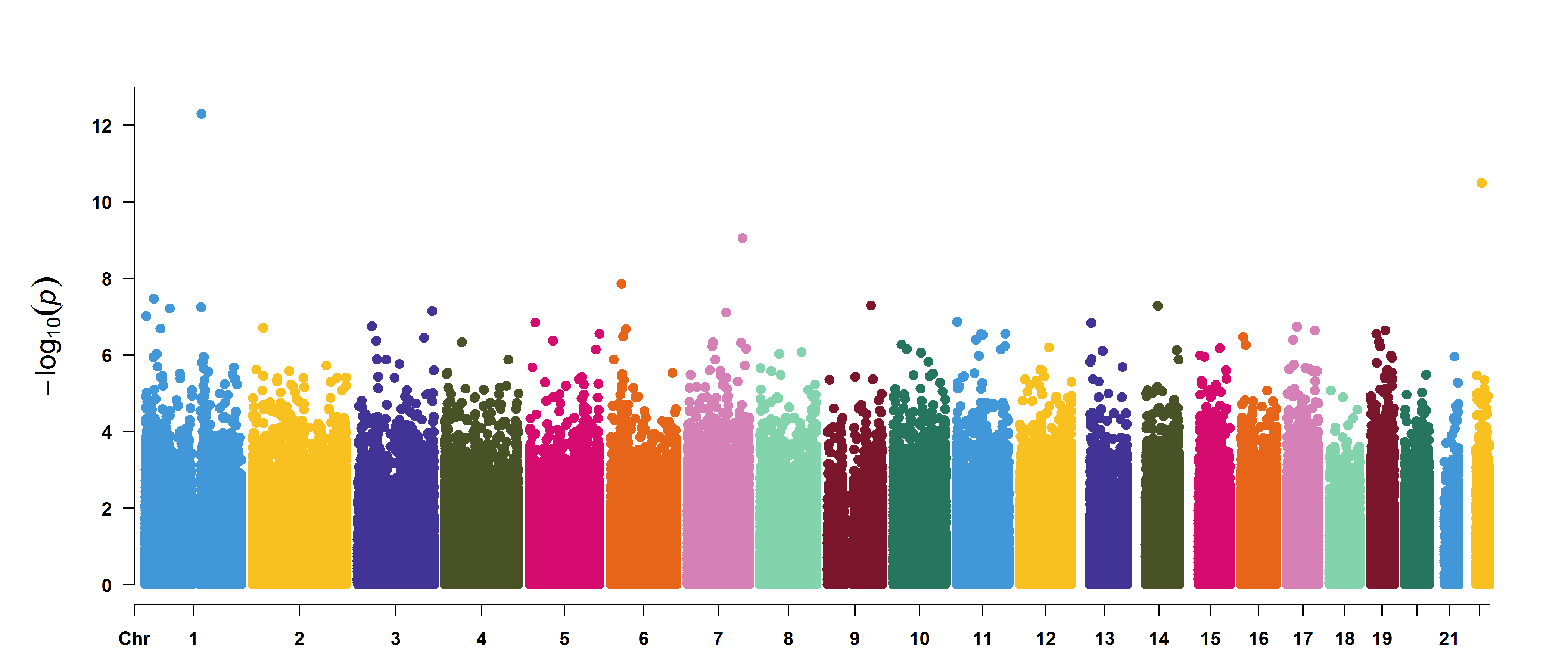
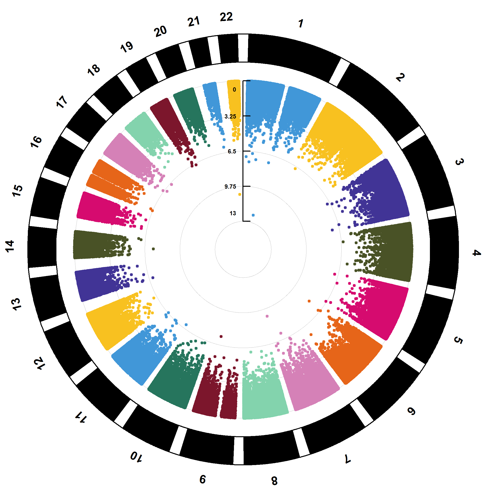
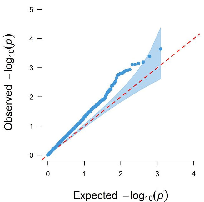
Option 1: EWAS results visualization
Visualize EWAS results based on the CMplot package,
including Manhattan plots, QQ plots, etc. The QQ plot is used to test
for genomic inflation, while the Manhattan plot is used to display EWAS
results. The user decides which to use for plotting based on the
parameter p: “PVAL”, “FDR”, or “Bonferroni”. Additionally,
the threshold parameter is used to plot a threshold line on
the Manhattan plot. Detailed information can be found at plotEWAS
documentation.
res <- plotEWAS(input = res,
                file = "pdf", # "jpg", "png", "tif", "pdf"
                p = "PVAL",   # "PVAL", "FDR", "Bonfferoni"
                threshold = 0.05)
#> EWAS Visualization has completed!
#> You can find results in D:/R/Rwork/Rpackage/easyEWAS/vignettes/EWASresult.
#> 2025-01-03 14:34:34.696527
#> 0.17 sec elapsed
Here are the example plots of the EWAS results.
Option 2: Internal validation with bootstrap
Bootstrap is a statistical resampling technique used for internal
validation and estimation of uncertainty in statistical models. The
parameterbootCI refers to the type of confidence interval
calculation methods, including “norm”, “basic”, “stud”, “perc” (the
default), and “bca”.Users can select CpG sites to validate in two ways.
One is to set the P-value column (PVAL, FDR, Bonfferoni) to be filtered
and its filtering cutoff value (default is 0.05).
res <- bootEWAS(input = res,
                filterP = "PVAL", # FDR, Bonferroni
                cutoff = 0.001,
                bootCI = "perc",
                times = 100)
#> Bootstrap analysis for cg01444397_BC11...
#> Bootstrap analysis for cg26269881_BC21...
#> Bootstrap analysis for cg08693699_BC21...
#> Bootstrap analysis for cg14151354_BC21...
#> Bootstrap analysis for cg13515269_TC21...
#> Bootstrap analysis for cg16047471_BC21...
#> Bootstrap analysis for cg00200653_TC11...
#> Bootstrap analysis for cg04162685_BC21...
#> Bootstrap analysis for cg24867447_BC21...
#> Bootstrap analysis for cg25069388_BC21...
#> Bootstrap for internal validation has been completed !
#> You can find results in D:/R/Rwork/Rpackage/easyEWAS/vignettes/EWASresult.
#> 2025-01-03 14:34:35.688672
#> 0.89 sec elapsed
The function ultimately provides the original statistical values for
each CpG site alongside their bootstrap-derived confidence intervals.
The result is stored in res$bootres.
head(res$bootres)
#> # A tibble: 6 × 4
#>   probe            original  lower_CI  upper_CI
#>   <chr>               <dbl>     <dbl>     <dbl>
#> 1 cg01444397_BC11  0.000572  0.000130  0.000977
#> 2 cg26269881_BC21 -0.00232  -0.00380  -0.000909
#> 3 cg08693699_BC21 -0.00113  -0.00168  -0.000397
#> 4 cg14151354_BC21 -0.000746 -0.00121  -0.000313
#> 5 cg13515269_TC21 -0.00135  -0.00224  -0.000679
#> 6 cg16047471_BC21 -0.00183  -0.00279  -0.000805
Another way is to specify the names of the sites to be validated
directly in the CpGs parameter. Here is an example (Not
run). Detailed information can be found at bootEWAS
documentation.
res <- bootEWAS(input = res,
                CpGs = "cg01444397_BC11,cg08693699_BC21,cg16047471_BC21",
                bootCI = "perc",
                times = 100)
Option 3: Enrichment analysis
easyEWAS provides two enrichment analysis methods (GO and KEGG) based
on the clusterProfiler package. Users can filter the
sites and their corresponding genes for enrichment analysis using the
filterP and cutoff parameters.The enrichment
methods include Gene Ontology (GO) and Kyoto Encyclopedia of Genes and
Genomes (KEGG). Within GO, there are three categories: Biological
Process (BP), Molecular Function (MF), and Cellular Component (CC).
Users can choose one or all categories for enrichment analysis, with BP
set as the default. Detailed information can be found at enrichEWAS
documentation.
res <- enrichEWAS(input = res,
                  method = "GO",
                  filterP = "PVAL",       # "PVAL", "FDR", "Bonfferoni"
                  cutoff = 0.01,
                  ont = "BP",             # "BP", "MF", "CC", "ALL"
                  plot = TRUE,
                  plotType = "dot",       # "bar", "dot"
                  plotcolor = "pvalue",   # "pvalue" or "p.adjust" or "qvalue"
                  showCategory = 10)
#> It will take some time, please be patient...
#> Start enrichment analysis ...
#> Start result visualization ...
#> Saving 7.29 x 4.51 in image
#> Enrichment analysis has been completed !
#> You can find results in D:/R/Rwork/Rpackage/easyEWAS/vignettes/EWASresult.
#> 2025-01-03 14:34:55.441067
#> 19.61 sec elapsed
The analysis results are stored in res$enrichresult.
head(res$enrichres)
#>                    ID
#> GO:0048511 GO:0048511
#> GO:0032922 GO:0032922
#> GO:0018107 GO:0018107
#> GO:0018210 GO:0018210
#> GO:2000058 GO:2000058
#> GO:0007623 GO:0007623
#>                                                            Description
#> GO:0048511                                            rhythmic process
#> GO:0032922                     circadian regulation of gene expression
#> GO:0018107                          peptidyl-threonine phosphorylation
#> GO:0018210                             peptidyl-threonine modification
#> GO:2000058 regulation of ubiquitin-dependent protein catabolic process
#> GO:0007623                                            circadian rhythm
#>            GeneRatio   BgRatio  RichFactor FoldEnrichment    zScore
#> GO:0048511       3/5 297/18888 0.010101010       38.15758 10.502803
#> GO:0032922       2/5  70/18888 0.028571429      107.93143 14.584739
#> GO:0018107       2/5  96/18888 0.020833333       78.70000 12.419415
#> GO:0018210       2/5 106/18888 0.018867925       71.27547 11.806381
#> GO:2000058       2/5 166/18888 0.012048193       45.51325  9.373424
#> GO:0007623       2/5 205/18888 0.009756098       36.85463  8.399045
#>                  pvalue    p.adjust      qvalue               geneID Count
#> GO:0048511 3.759965e-05 0.009099115 0.003285022 PER3/BHLHE41/CSNK2A1     3
#> GO:0032922 1.344212e-04 0.016264968 0.005872085         PER3/BHLHE41     2
#> GO:0018107 2.531146e-04 0.018668599 0.006739860       PRKAG2/CSNK2A1     2
#> GO:0018210 3.085719e-04 0.018668599 0.006739860       PRKAG2/CSNK2A1     2
#> GO:2000058 7.545427e-04 0.036519868 0.013184641      CSNK1A1/CSNK2A1     2
#> GO:0007623 1.147290e-03 0.037627614 0.013584567         PER3/BHLHE41     2
Additionally, the function can visualize the enrichment analysis
results, including both dotplot and barplot. The colors in the plot can
be based on the values of pvalue, p.adjust, or qvalue, with pvalue being
the default. Here, we can obtain a bubble plot of GO enrichment
analysis.

Option 4: DMR analysis
The easyEWAS package integrates the DMRcate method
to support DMR analysis. Similar to DMP analysis, users need to specify
the exposure variable and covariates for DMR analysis, as well as the
chip type and methylation value type (β-values or M-values). It is
recommended to use the default settings for parameters such as
lambda, C, fdrCPG,
pcutoff, and min.cpgs for DMR selection. Here,
since there are too few significant DMRs, the pcutoff is
set to 0.05 (Default to “fdr”). For detailed information on these
parameters, please refer to dmrEWAS
documentation.
res <- dmrEWAS(input = res,
               chipType = "EPICV2",
               what = "Beta",
               expo = "var",
               cov = "cov1,cov2",
               genome = "hg38",
               lambda=1000,
               C = 2,
               pcutoff = 0.05
)
#> Filtering out position replicates from an EPICv2 beta- or M-matrix. Please be patient...
#> Starting the differentially methylated region analysis. Please be patient...
#> Differentially Methylated Region analysis has been completed!
#> You can find results in D:/R/Rwork/Rpackage/easyEWAS/vignettes/EWASresult.
#> 2025-01-03 14:35:52.345173
#> 56.8 sec elapsed
The result is stored in res$dmrres.
head(res$dmrres)
#>   seqnames     start       end width strand no.cpgs min_smoothed_fdr
#> 1    chr12  26121435  26121868   434      *       3     0.0006926403
#> 2     chr1   7826573   7827921  1349      *      10     0.0053198587
#> 3     chr1   7784390   7784835   446      *       4     0.0053198587
#> 4     chr3   4981365   4981709   345      *       3     0.0054574766
#> 5     chr2 100924866 100925130   265      *       5     0.0081198870
#> 6    chr15  60591026  60591370   345      *       2     0.0081198870
#>       Stouffer       HMFDR       Fisher      maxdiff      meandiff
#> 1 2.827015e-04 0.002443061 0.0001300913 -0.001834445 -0.0011539964
#> 2 6.166338e-06 0.039505450 0.0001300913 -0.002527727 -0.0012950516
#> 3 4.259913e-03 0.003212979 0.0007271626  0.002012009  0.0006847355
#> 4 3.654183e-04 0.003212979 0.0007015946 -0.002322104 -0.0015218217
#> 5 3.580945e-04 0.016418020 0.0007015946 -0.002072670 -0.0013957993
#> 6 1.749110e-03 0.003092856 0.0013320402 -0.001368543 -0.0006471749
#>   overlapping.genes
#> 1           BHLHE41
#> 2    PER3, Z98884.1
#> 3              PER3
#> 4           BHLHE40
#> 5             NPAS2
#> 6    RORA-AS1, RORA
Reference
1. Hall P (1992). The Bootstrap and Edgeworth
Expansion. Springer, New York. ISBN 9781461243847.
2. https://CRAN.R-project.org/package=CMplot
3. Yu, G., Wang, L. G., Han, Y., & He, Q. Y.
(2012). clusterProfiler: an R package for comparing biological themes
among gene clusters. Omics : a journal of integrative biology, 16(5),
284–287. https://doi.org/10.1089/omi.2011.0118
4. Leek, J. T., Johnson, W. E., Parker, H. S., Jaffe,
A. E., & Storey, J. D. (2012). The sva package for removing batch
effects and other unwanted variation in high-throughput experiments.
Bioinformatics (Oxford, England), 28(6), 882–883. https://doi.org/10.1093/bioinformatics/bts034
5. Peters, T. J., Buckley, M. J., Statham, A. L.,
Pidsley, R., Samaras, K., V Lord, R., Clark, S. J., & Molloy, P. L.
(2015). De novo identification of differentially methylated regions in
the human genome. Epigenetics & chromatin, 8, 6. https://doi.org/10.1186/1756-8935-8-6